注意
前往末尾 以下载完整示例代码。
Logit 刻度#
使用 Logit 坐标轴的图表示例。
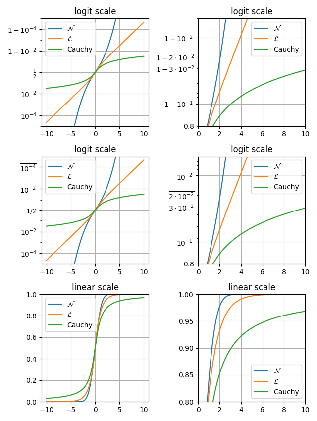
本示例展示了 set_yscale("logit") 如何在概率图上工作,通过在一个图中生成三种分布:正态分布、拉普拉斯分布和柯西分布。
Logit 刻度的优点在于它能有效地展开接近 0 和 1 的值。
在线性刻度图中,接近 0 和 1 的概率值显得非常压缩,使得难以分辨这些区域的差异。
在 Logit 刻度图中,这种转换扩展了这些区域,使图表更清晰,并且更容易比较不同概率值之间的差异。
这使得 Logit 刻度在可视化逻辑回归、分类模型和累积分布函数中的概率时特别有用。
import math

import matplotlib.pyplot as plt
import numpy as np

xmax = 10
x = np.linspace(-xmax, xmax, 10000)
cdf_norm = [math.erf(w / np.sqrt(2)) / 2 + 1 / 2 for w in x]
cdf_laplacian = np.where(x < 0, 1 / 2 * np.exp(x), 1 - 1 / 2 * np.exp(-x))
cdf_cauchy = np.arctan(x) / np.pi + 1 / 2

fig, axs = plt.subplots(nrows=3, ncols=2, figsize=(6.4, 8.5))

# Common part, for the example, we will do the same plots on all graphs
for i in range(3):
    for j in range(2):
        axs[i, j].plot(x, cdf_norm, label=r"$\mathcal{N}$")
        axs[i, j].plot(x, cdf_laplacian, label=r"$\mathcal{L}$")
        axs[i, j].plot(x, cdf_cauchy, label="Cauchy")
        axs[i, j].legend()
        axs[i, j].grid()

# First line, logitscale, with standard notation
axs[0, 0].set(title="logit scale")
axs[0, 0].set_yscale("logit")
axs[0, 0].set_ylim(1e-5, 1 - 1e-5)

axs[0, 1].set(title="logit scale")
axs[0, 1].set_yscale("logit")
axs[0, 1].set_xlim(0, xmax)
axs[0, 1].set_ylim(0.8, 1 - 5e-3)

# Second line, logitscale, with survival notation (with `use_overline`), and
# other format display 1/2
axs[1, 0].set(title="logit scale")
axs[1, 0].set_yscale("logit", one_half="1/2", use_overline=True)
axs[1, 0].set_ylim(1e-5, 1 - 1e-5)

axs[1, 1].set(title="logit scale")
axs[1, 1].set_yscale("logit", one_half="1/2", use_overline=True)
axs[1, 1].set_xlim(0, xmax)
axs[1, 1].set_ylim(0.8, 1 - 5e-3)

# Third line, linear scale
axs[2, 0].set(title="linear scale")
axs[2, 0].set_ylim(0, 1)

axs[2, 1].set(title="linear scale")
axs[2, 1].set_xlim(0, xmax)
axs[2, 1].set_ylim(0.8, 1)

fig.tight_layout()
plt.show()
脚本总运行时间: (0 分 2.391 秒)