带有误差带的曲线

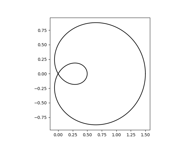
此示例演示了如何围绕参数化曲线绘制误差带。

可以使用plot直接绘制参数化曲线 x(t), y(t)。

import matplotlib.pyplot as plt
import numpy as np

from matplotlib.patches import PathPatch
from matplotlib.path import Path

N = 400
t = np.linspace(0, 2 * np.pi, N)
r = 0.5 + np.cos(t)
x, y = r * np.cos(t), r * np.sin(t)

fig, ax = plt.subplots()
ax.plot(x, y, "k")
ax.set(aspect=1)

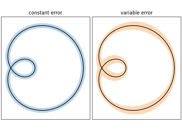
误差带可用于指示曲线的不确定性。在此示例中，我们假设误差可以表示为一个标量 err，它描述了曲线在每个点处垂直方向上的不确定性。

我们使用PathPatch将此误差可视化为路径周围的彩色带。该补丁由两个路径段 (xp, yp) 和 (xn, yn) 创建，它们相对于曲线 (x, y) 沿垂直方向平移 +/- err。

注意：使用PathPatch的这种方法适用于二维中的任意曲线。如果您只是一个标准的y-x散点图，您可以使用更简单的fill_between方法（另请参见填充两条线之间的区域）。

def draw_error_band(ax, x, y, err, **kwargs):
    # Calculate normals via centered finite differences (except the first point
    # which uses a forward difference and the last point which uses a backward
    # difference).
    dx = np.concatenate([[x[1] - x[0]], x[2:] - x[:-2], [x[-1] - x[-2]]])
    dy = np.concatenate([[y[1] - y[0]], y[2:] - y[:-2], [y[-1] - y[-2]]])
    l = np.hypot(dx, dy)
    nx = dy / l
    ny = -dx / l

    # end points of errors
    xp = x + nx * err
    yp = y + ny * err
    xn = x - nx * err
    yn = y - ny * err

    vertices = np.block([[xp, xn[::-1]],
                         [yp, yn[::-1]]]).T
    codes = np.full(len(vertices), Path.LINETO)
    codes[0] = codes[len(xp)] = Path.MOVETO
    path = Path(vertices, codes)
    ax.add_patch(PathPatch(path, **kwargs))


_, axs = plt.subplots(1, 2, layout='constrained', sharex=True, sharey=True)
errs = [
    (axs[0], "constant error", 0.05),
    (axs[1], "variable error", 0.05 * np.sin(2 * t) ** 2 + 0.04),
]
for i, (ax, title, err) in enumerate(errs):
    ax.set(title=title, aspect=1, xticks=[], yticks=[])
    ax.plot(x, y, "k")
    draw_error_band(ax, x, y, err=err,
                    facecolor=f"C{i}", edgecolor="none", alpha=.3)

plt.show()

参考

本示例展示了以下函数、方法、类和模块的使用

• matplotlib.patches.PathPatch

• matplotlib.path.Path

标签： 组件：误差 绘图类型：线条 级别：中等