在地图上绘制数据(示例集)
以下一系列示例将说明如何使用 Basemap 实例方法在地图上绘制数据。更多示例包含在 basemap 源代码分发包的 doc/examples 目录中。有多种 Basemap 实例方法可用于绘制数据:
contour(): 绘制等高线。contourf(): 绘制填充等高线。imshow(): 绘制图像。pcolor(): 绘制伪彩色图。pcolormesh(): 绘制伪彩色图(规则网格的更快版本)。plot(): 绘制线条和/或标记。scatter(): 绘制带标记的点。quiver(): 绘制向量。drawgreatcircle(): 绘制大圆。
这些实例方法中的许多只是将调用转发给相应的 Matplotlib Axes 实例方法,并进行一些额外的预处理/后处理和参数检查。您还可以使用 Matplotlib pyplot 接口或面向对象 API,直接在地图上绘图,方法是使用与 Basemap 相关联的 Axes 实例。
有关如何使用 Basemap 实例方法的更多详细信息,请参阅 Basemap API。
以下是示例(其中许多利用 netcdf4-python 模块通过 HTTP 获取数据集)
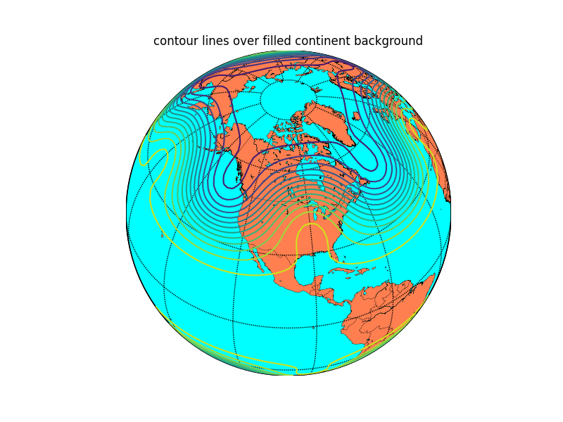
在 Basemap 上绘制等高线
from mpl_toolkits.basemap import Basemap
import matplotlib.pyplot as plt
import numpy as np
# set up orthographic map projection with
# perspective of satellite looking down at 45N, 100W.
# use low resolution coastlines.
map = Basemap(projection='ortho',lat_0=45,lon_0=-100,resolution='l')
# draw coastlines, country boundaries, fill continents.
map.drawcoastlines(linewidth=0.25)
map.drawcountries(linewidth=0.25)
map.fillcontinents(color='coral',lake_color='aqua')
# draw the edge of the map projection region (the projection limb)
map.drawmapboundary(fill_color='aqua')
# draw lat/lon grid lines every 30 degrees.
map.drawmeridians(np.arange(0,360,30))
map.drawparallels(np.arange(-90,90,30))
# make up some data on a regular lat/lon grid.
nlats = 73; nlons = 145; delta = 2.*np.pi/(nlons-1)
lats = (0.5*np.pi-delta*np.indices((nlats,nlons))[0,:,:])
lons = (delta*np.indices((nlats,nlons))[1,:,:])
wave = 0.75*(np.sin(2.*lats)**8*np.cos(4.*lons))
mean = 0.5*np.cos(2.*lats)*((np.sin(2.*lats))**2 + 2.)
# compute native map projection coordinates of lat/lon grid.
x, y = map(lons*180./np.pi, lats*180./np.pi)
# contour data over the map.
cs = map.contour(x,y,wave+mean,15,linewidths=1.5)
plt.title('contour lines over filled continent background')
plt.show()
(源代码)
绘制带填充等高线的降水图
from mpl_toolkits.basemap import Basemap, cm
# requires netcdf4-python (netcdf4-python.googlecode.com)
from netCDF4 import Dataset as NetCDFFile
import os
import numpy as np
import matplotlib.pyplot as plt

# plot rainfall from NWS using special precipitation
# colormap used by the NWS, and included in basemap.

ncpath = os.path.join(*3 * [".."] + ["examples", "nws_precip_conus_20061222.nc"])
nc = NetCDFFile(ncpath)
# data from http://water.weather.gov/precip/
prcpvar = nc.variables['amountofprecip']
data = 0.01*prcpvar[:]
latcorners = nc.variables['lat'][:]
loncorners = -nc.variables['lon'][:]
lon_0 = -nc.variables['true_lon'].getValue()
lat_0 = nc.variables['true_lat'].getValue()
# create figure and axes instances
fig = plt.figure(figsize=(8,8))
ax = fig.add_axes([0.1,0.1,0.8,0.8])
# create polar stereographic Basemap instance.
m = Basemap(projection='stere',lon_0=lon_0,lat_0=90.,lat_ts=lat_0,\
            llcrnrlat=latcorners[0],urcrnrlat=latcorners[2],\
            llcrnrlon=loncorners[0],urcrnrlon=loncorners[2],\
            rsphere=6371200.,resolution='l',area_thresh=10000)
# draw coastlines, state and country boundaries, edge of map.
m.drawcoastlines()
m.drawstates()
m.drawcountries()
# draw parallels.
parallels = np.arange(0.,90,10.)
m.drawparallels(parallels,labels=[1,0,0,0],fontsize=10)
# draw meridians
meridians = np.arange(180.,360.,10.)
m.drawmeridians(meridians,labels=[0,0,0,1],fontsize=10)
ny = data.shape[0]; nx = data.shape[1]
lons, lats = m.makegrid(nx, ny) # get lat/lons of ny by nx evenly space grid.
x, y = m(lons, lats) # compute map proj coordinates.
# draw filled contours.
clevs = [0,1,2.5,5,7.5,10,15,20,30,40,50,70,100,150,200,250,300,400,500,600,750]
cs = m.contourf(x,y,data,clevs,cmap=cm.s3pcpn)
# add colorbar.
cbar = m.colorbar(cs,location='bottom',pad="5%")
cbar.set_label('mm')
# add title
plt.title(prcpvar.long_name+' for period ending '+prcpvar.dateofdata)
plt.show()
(源代码)
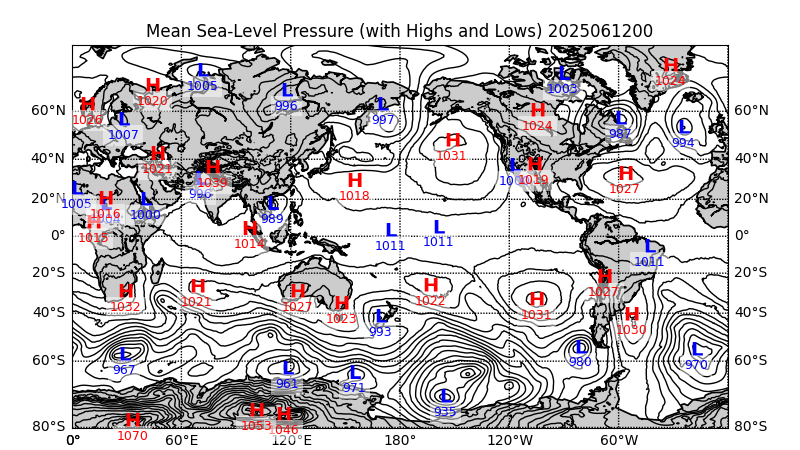
绘制带有高压和低压标记的海平面气压天气图
"""
plot H's and L's on a sea-level pressure map
(uses scipy.ndimage.filters and netcdf4-python)
"""
import datetime as dt
import numpy as np
import matplotlib.pyplot as plt
from mpl_toolkits.basemap import Basemap, addcyclic
from scipy.ndimage.filters import minimum_filter, maximum_filter
from netCDF4 import Dataset


def extrema(mat,mode='wrap',window=10):
    """find the indices of local extrema (min and max)
    in the input array."""
    mn = minimum_filter(mat, size=window, mode=mode)
    mx = maximum_filter(mat, size=window, mode=mode)
    # (mat == mx) true if pixel is equal to the local max
    # (mat == mn) true if pixel is equal to the local in
    # Return the indices of the maxima, minima
    return np.nonzero(mat == mn), np.nonzero(mat == mx)


# Plot 00 UTC yesterday.
url = "http://nomads.ncep.noaa.gov/dods/gfs_0p50/gfs%Y%m%d/gfs_0p50_00z"
date = dt.datetime.now() - dt.timedelta(days=1)

# open OpenDAP dataset.
data = Dataset(date.strftime(url))

# read lats,lons.
lats = data.variables['lat'][:]
lons1 = data.variables['lon'][:]
nlats = len(lats)
nlons = len(lons1)
# read prmsl, convert to hPa (mb).
prmsl = 0.01*data.variables['prmslmsl'][0]
# the window parameter controls the number of highs and lows detected.
# (higher value, fewer highs and lows)
local_min, local_max = extrema(prmsl, mode='wrap', window=50)
# create Basemap instance.
m =\
Basemap(llcrnrlon=0,llcrnrlat=-80,urcrnrlon=360,urcrnrlat=80,projection='mill')
# add wrap-around point in longitude.
prmsl, lons = addcyclic(prmsl, lons1)
# contour levels
clevs = np.arange(900,1100.,5.)
# find x,y of map projection grid.
lons, lats = np.meshgrid(lons, lats)
x, y = m(lons, lats)
# create figure.
fig=plt.figure(figsize=(8,4.5))
ax = fig.add_axes([0.05,0.05,0.9,0.85])
cs = m.contour(x,y,prmsl,clevs,colors='k',linewidths=1.)
m.drawcoastlines(linewidth=1.25)
m.fillcontinents(color='0.8')
m.drawparallels(np.arange(-80,81,20),labels=[1,1,0,0])
m.drawmeridians(np.arange(0,360,60),labels=[0,0,0,1])
xlows = x[local_min]; xhighs = x[local_max]
ylows = y[local_min]; yhighs = y[local_max]
lowvals = prmsl[local_min]; highvals = prmsl[local_max]
# plot lows as blue L's, with min pressure value underneath.
xyplotted = []
# don't plot if there is already a L or H within dmin meters.
yoffset = 0.022*(m.ymax-m.ymin)
dmin = yoffset
for x,y,p in zip(xlows, ylows, lowvals):
    if x < m.xmax and x > m.xmin and y < m.ymax and y > m.ymin:
        dist = [np.sqrt((x-x0)**2+(y-y0)**2) for x0,y0 in xyplotted]
        if not dist or min(dist) > dmin:
            plt.text(x,y,'L',fontsize=14,fontweight='bold',
                    ha='center',va='center',color='b')
            plt.text(x,y-yoffset,repr(int(p)),fontsize=9,
                    ha='center',va='top',color='b',
                    bbox = dict(boxstyle="square",ec='None',fc=(1,1,1,0.5)))
            xyplotted.append((x,y))
# plot highs as red H's, with max pressure value underneath.
xyplotted = []
for x,y,p in zip(xhighs, yhighs, highvals):
    if x < m.xmax and x > m.xmin and y < m.ymax and y > m.ymin:
        dist = [np.sqrt((x-x0)**2+(y-y0)**2) for x0,y0 in xyplotted]
        if not dist or min(dist) > dmin:
            plt.text(x,y,'H',fontsize=14,fontweight='bold',
                    ha='center',va='center',color='r')
            plt.text(x,y-yoffset,repr(int(p)),fontsize=9,
                    ha='center',va='top',color='r',
                    bbox = dict(boxstyle="square",ec='None',fc=(1,1,1,0.5)))
            xyplotted.append((x,y))

datestr = date.strftime("%Y%m%d00")
plt.title('Mean Sea-Level Pressure (with Highs and Lows) %s' % datestr)
plt.show()
(源代码)
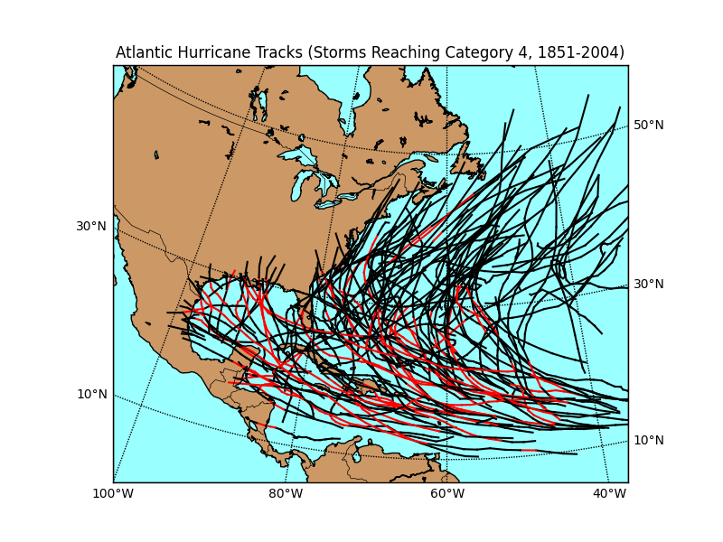
从 Shapefile 绘制飓风路径
"""
draw Atlantic Hurricane Tracks for storms that reached Cat 4 or 5.
part of the track for which storm is cat 4 or 5 is shown red.
ESRI shapefile data from http://nationalatlas.gov/mld/huralll.html
"""
import os
import numpy as np
import matplotlib.pyplot as plt
from mpl_toolkits.basemap import Basemap
# Lambert Conformal Conic map.
m = Basemap(llcrnrlon=-100.,llcrnrlat=0.,urcrnrlon=-20.,urcrnrlat=57.,
            projection='lcc',lat_1=20.,lat_2=40.,lon_0=-60.,
            resolution ='l',area_thresh=1000.)
# read shapefile.
shp_path = os.path.join(*3 * [".."] + ["examples", "huralll020"])
shp_info = m.readshapefile(shp_path,'hurrtracks',drawbounds=False)
# find names of storms that reached Cat 4.
names = []
for shapedict in m.hurrtracks_info:
    cat = shapedict['CATEGORY']
    name = shapedict['NAME']
    if cat in ['H4','H5'] and name not in names:
        # only use named storms.
        if name != 'NOT NAMED':  names.append(name)
# plot tracks of those storms.
for shapedict,shape in zip(m.hurrtracks_info,m.hurrtracks):
    name = shapedict['NAME']
    cat = shapedict['CATEGORY']
    if name in names:
        xx,yy = zip(*shape)
        # show part of track where storm > Cat 4 as thick red.
        if cat in ['H4','H5']:
            m.plot(xx,yy,linewidth=1.5,color='r')
        elif cat in ['H1','H2','H3']:
            m.plot(xx,yy,color='k')
# draw coastlines, meridians and parallels.
m.drawcoastlines()
m.drawcountries()
m.drawmapboundary(fill_color='#99ffff')
m.fillcontinents(color='#cc9966',lake_color='#99ffff')
m.drawparallels(np.arange(10,70,20),labels=[1,1,0,0])
m.drawmeridians(np.arange(-100,0,20),labels=[0,0,0,1])
plt.title('Atlantic Hurricane Tracks (Storms Reaching Category 4, 1851-2004)')
plt.show()
(源代码)
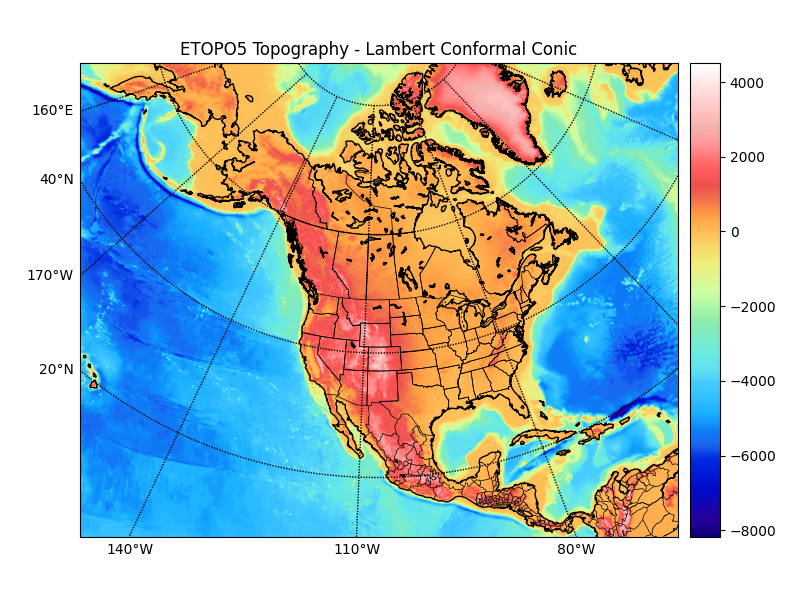
将 etopo5 地形/水深测量数据绘制为图像(带或不带指定光源的阴影)。
from mpl_toolkits.basemap import Basemap, shiftgrid, cm
import numpy as np
import matplotlib.pyplot as plt
from netCDF4 import Dataset

# read in etopo5 topography/bathymetry.
url = 'http://ferret.pmel.noaa.gov/thredds/dodsC/data/PMEL/etopo5.nc'
etopodata = Dataset(url)

topoin = etopodata.variables['ROSE'][:]
lons = etopodata.variables['ETOPO05_X'][:]
lats = etopodata.variables['ETOPO05_Y'][:]
# shift data so lons go from -180 to 180 instead of 20 to 380.
topoin,lons = shiftgrid(180.,topoin,lons,start=False)

# plot topography/bathymetry as an image.

# create the figure and axes instances.
fig = plt.figure()
ax = fig.add_axes([0.1,0.1,0.8,0.8])
# setup of basemap ('lcc' = lambert conformal conic).
# use major and minor sphere radii from WGS84 ellipsoid.
m = Basemap(llcrnrlon=-145.5,llcrnrlat=1.,urcrnrlon=-2.566,urcrnrlat=46.352,\
            rsphere=(6378137.00,6356752.3142),\
            resolution='l',area_thresh=1000.,projection='lcc',\
            lat_1=50.,lon_0=-107.,ax=ax)
# transform to nx x ny regularly spaced 5km native projection grid
nx = int((m.xmax-m.xmin)/5000.)+1; ny = int((m.ymax-m.ymin)/5000.)+1
topodat = m.transform_scalar(topoin,lons,lats,nx,ny)
# plot image over map with imshow.
im = m.imshow(topodat,cm.GMT_haxby)
# draw coastlines and political boundaries.
m.drawcoastlines()
m.drawcountries()
m.drawstates()
# draw parallels and meridians.
# label on left and bottom of map.
parallels = np.arange(0.,80,20.)
m.drawparallels(parallels,labels=[1,0,0,1])
meridians = np.arange(10.,360.,30.)
m.drawmeridians(meridians,labels=[1,0,0,1])
# add colorbar
cb = m.colorbar(im,"right", size="5%", pad='2%')
ax.set_title('ETOPO5 Topography - Lambert Conformal Conic')
plt.show()
(源代码)
# make a shaded relief plot.

# create new figure, axes instance.
fig = plt.figure()
ax = fig.add_axes([0.1,0.1,0.8,0.8])
# attach new axes image to existing Basemap instance.
m.ax = ax
# create light source object.
from matplotlib.colors import LightSource
ls = LightSource(azdeg = 90, altdeg = 20)
# convert data to rgb array including shading from light source.
# (must specify color map)
rgb = ls.shade(topodat, cm.GMT_haxby)
im = m.imshow(rgb)
# draw coastlines and political boundaries.
m.drawcoastlines()
m.drawcountries()
m.drawstates()
ax.set_title('Shaded ETOPO5 Topography - Lambert Conformal Conic')
plt.show()
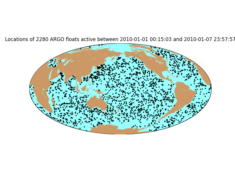
在 ARGO 浮标位置绘制标记。
from netCDF4 import Dataset, num2date
import time, calendar, datetime, numpy
from mpl_toolkits.basemap import Basemap
import matplotlib.pyplot as plt
import os
try:
    from urllib.request import urlretrieve
except ImportError:
    from urllib import urlretrieve
# data downloaded from the form at
# http://coastwatch.pfeg.noaa.gov/erddap/tabledap/apdrcArgoAll.html
filename, headers = urlretrieve("https://erddap.ifremer.fr/erddap/tabledap/ArgoFloats-index.nc?date%2Clatitude%2Clongitude&date%3E=2010-01-01&date%3C=2010-01-08&latitude%3E=-90&latitude%3C=90&longitude%3E=-180&longitude%3C=180&distinct()")
dset = Dataset(filename)
lats = dset.variables['latitude'][:]
lons = dset.variables['longitude'][:]
time = dset.variables['date']  # seconds since epoch
times = time[:]
t1 = times.min(); t2 = times.max()
date1 = num2date(t1, units=time.units)
date2 = num2date(t2, units=time.units)
dset.close()
os.remove(filename)
# draw map with markers for float locations
m = Basemap(projection='hammer',lon_0=180)
x, y = m(lons,lats)
m.drawmapboundary(fill_color='#99ffff')
m.fillcontinents(color='#cc9966',lake_color='#99ffff')
m.scatter(x,y,3,marker='o',color='k')
plt.title('Locations of %s ARGO floats active between %s and %s' %\
        (len(lats),date1,date2),fontsize=12)
plt.show()
(源代码)
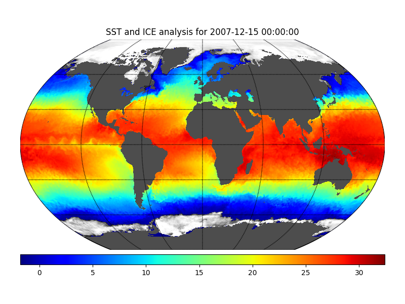
SST 和海冰分析的伪彩色图。
from mpl_toolkits.basemap import Basemap
from netCDF4 import Dataset, date2index
import numpy as np
import matplotlib.pyplot as plt
from datetime import datetime
try:
    from urllib.request import urlretrieve
except ImportError:
    from urllib import urlretrieve
date = datetime(2007,12,15,0) # date to plot.
# open dataset.
sstpath, sstheader = urlretrieve("https://downloads.psl.noaa.gov/Datasets/noaa.oisst.v2.highres/sst.day.mean.{0}.nc".format(date.year))
dataset = Dataset(sstpath)
timevar = dataset.variables['time']
timeindex = date2index(date,timevar) # find time index for desired date.
# read sst.  Will automatically create a masked array using
# missing_value variable attribute. 'squeeze out' singleton dimensions.
sst = dataset.variables['sst'][timeindex,:].squeeze()
# read ice.
dataset.close()
icepath, iceheader = urlretrieve("https://downloads.psl.noaa.gov/Datasets/noaa.oisst.v2.highres/icec.day.mean.{0}.nc".format(date.year))
dataset = Dataset(icepath)
ice = dataset.variables['icec'][timeindex,:].squeeze()
# read lats and lons (representing centers of grid boxes).
lats = dataset.variables['lat'][:]
lons = dataset.variables['lon'][:]
dataset.close()
latstep, lonstep = np.diff(lats[:2]), np.diff(lons[:2])
lats = np.append(lats - 0.5 * latstep, lats[-1] + 0.5 * latstep)
lons = np.append(lons - 0.5 * lonstep, lons[-1] + 0.5 * lonstep)
lons, lats = np.meshgrid(lons,lats)
# create figure, axes instances.
fig = plt.figure()
ax = fig.add_axes([0.05,0.05,0.9,0.9])
# create Basemap instance.
# coastlines not used, so resolution set to None to skip
# continent processing (this speeds things up a bit)
m = Basemap(projection='kav7',lon_0=0,resolution=None)
# draw line around map projection limb.
# color background of map projection region.
# missing values over land will show up this color.
m.drawmapboundary(fill_color='0.3')
# plot sst, then ice with pcolor
im1 = m.pcolormesh(lons,lats,sst,shading='flat',cmap=plt.cm.jet,latlon=True)
im2 = m.pcolormesh(lons,lats,ice,shading='flat',cmap=plt.cm.gist_gray,latlon=True)
# draw parallels and meridians, but don't bother labelling them.
m.drawparallels(np.arange(-90.,99.,30.))
m.drawmeridians(np.arange(-180.,180.,60.))
# add colorbar
cb = m.colorbar(im1,"bottom", size="5%", pad="2%")
# add a title.
ax.set_title('SST and ICE analysis for %s'%date)
plt.show()
(源代码)
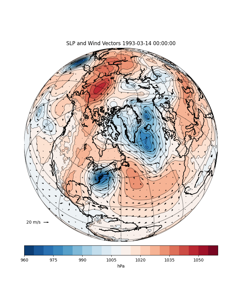
绘制风矢量和风羽。
import numpy as np
import matplotlib.pyplot as plt
import datetime
from mpl_toolkits.basemap import Basemap, shiftgrid
from netCDF4 import Dataset
# specify date to plot.
yyyy=1993; mm=3; dd=14; hh=0
date = datetime.datetime(yyyy,mm,dd,hh)
# set OpenDAP server URL.
URLbase="https://www.ncei.noaa.gov/thredds/dodsC/model-cfs_reanl_6h_pgb/"
URL=URLbase+"%04i/%04i%02i/%04i%02i%02i/pgbh00.gdas.%04i%02i%02i%02i.grb2" %\
             (yyyy,yyyy,mm,yyyy,mm,dd,yyyy,mm,dd,hh)
data = Dataset(URL)
# read lats,lons
# reverse latitudes so they go from south to north.
latitudes = data.variables['lat'][::-1]
longitudes = data.variables['lon'][:].tolist()
# get sea level pressure and 10-m wind data.
# mult slp by 0.01 to put in units of hPa.
slpin = 0.01*data.variables['Pressure_msl'][:].squeeze()
uin = data.variables['u-component_of_wind_height_above_ground'][:].squeeze()
vin = data.variables['v-component_of_wind_height_above_ground'][:].squeeze()
# add cyclic points manually (could use addcyclic function)
slp = np.zeros((slpin.shape[0],slpin.shape[1]+1),np.float64)
slp[:,0:-1] = slpin[::-1]; slp[:,-1] = slpin[::-1,0]
u = np.zeros((uin.shape[0],uin.shape[1]+1),np.float64)
u[:,0:-1] = uin[::-1]; u[:,-1] = uin[::-1,0]
v = np.zeros((vin.shape[0],vin.shape[1]+1),np.float64)
v[:,0:-1] = vin[::-1]; v[:,-1] = vin[::-1,0]
longitudes.append(360.); longitudes = np.array(longitudes)
# make 2-d grid of lons, lats
lons, lats = np.meshgrid(longitudes,latitudes)
# make orthographic basemap.
m = Basemap(resolution='c',projection='ortho',lat_0=60.,lon_0=-60.)
# create figure, add axes
fig1 = plt.figure(figsize=(8,10))
ax = fig1.add_axes([0.1,0.1,0.8,0.8])
# set desired contour levels.
clevs = np.arange(960,1061,5)
# compute native x,y coordinates of grid.
x, y = m(lons, lats)
# define parallels and meridians to draw.
parallels = np.arange(-80.,90,20.)
meridians = np.arange(0.,360.,20.)
# plot SLP contours.
CS1 = m.contour(x,y,slp,clevs,linewidths=0.5,colors='k')
CS2 = m.contourf(x,y,slp,clevs,cmap=plt.cm.RdBu_r)
# plot wind vectors on projection grid.
# first, shift grid so it goes from -180 to 180 (instead of 0 to 360
# in longitude).  Otherwise, interpolation is messed up.
ugrid,newlons = shiftgrid(180.,u,longitudes,start=False)
vgrid,newlons = shiftgrid(180.,v,longitudes,start=False)
# transform vectors to projection grid.
uproj,vproj,xx,yy = \
m.transform_vector(ugrid,vgrid,newlons,latitudes,31,31,returnxy=True,masked=True)
# now plot.
Q = m.quiver(xx,yy,uproj,vproj,scale=700)
# make quiver key.
qk = plt.quiverkey(Q, 0.1, 0.1, 20, '20 m/s', labelpos='W')
# draw coastlines, parallels, meridians.
m.drawcoastlines(linewidth=1.5)
m.drawparallels(parallels)
m.drawmeridians(meridians)
# add colorbar
cb = m.colorbar(CS2,"bottom", size="5%", pad="2%")
cb.set_label('hPa')
# set plot title
ax.set_title('SLP and Wind Vectors '+str(date))
plt.show()
(源代码)
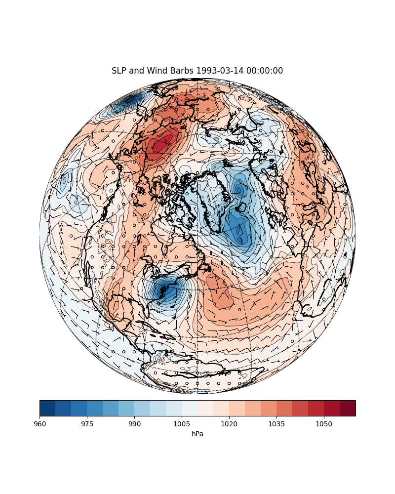
# create 2nd figure, add axes
fig2 = plt.figure(figsize=(8,10))
ax = fig2.add_axes([0.1,0.1,0.8,0.8])
# plot SLP contours
CS1 = m.contour(x,y,slp,clevs,linewidths=0.5,colors='k')
CS2 = m.contourf(x,y,slp,clevs,cmap=plt.cm.RdBu_r)
# plot wind barbs over map.
barbs = m.barbs(xx,yy,uproj,vproj,length=5,barbcolor='k',flagcolor='r',linewidth=0.5)
# draw coastlines, parallels, meridians.
m.drawcoastlines(linewidth=1.5)
m.drawparallels(parallels)
m.drawmeridians(meridians)
# add colorbar
cb = m.colorbar(CS2,"bottom", size="5%", pad="2%")
cb.set_label('hPa')
# set plot title.
ax.set_title('SLP and Wind Barbs '+str(date))
plt.show()
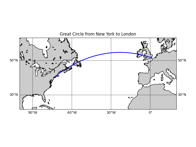
绘制纽约和伦敦之间的大圆。
from mpl_toolkits.basemap import Basemap
import numpy as np
import matplotlib.pyplot as plt
# create new figure, axes instances.
fig=plt.figure()
ax=fig.add_axes([0.1,0.1,0.8,0.8])
# setup mercator map projection.
m = Basemap(llcrnrlon=-100.,llcrnrlat=20.,urcrnrlon=20.,urcrnrlat=60.,\
            rsphere=(6378137.00,6356752.3142),\
            resolution='l',projection='merc',\
            lat_0=40.,lon_0=-20.,lat_ts=20.)
# nylat, nylon are lat/lon of New York
nylat = 40.78; nylon = -73.98
# lonlat, lonlon are lat/lon of London.
lonlat = 51.53; lonlon = 0.08
# draw great circle route between NY and London
m.drawgreatcircle(nylon,nylat,lonlon,lonlat,linewidth=2,color='b')
m.drawcoastlines()
m.fillcontinents()
# draw parallels
m.drawparallels(np.arange(10,90,20),labels=[1,1,0,1])
# draw meridians
m.drawmeridians(np.arange(-180,180,30),labels=[1,1,0,1])
ax.set_title('Great Circle from New York to London')
plt.show()
(源代码)
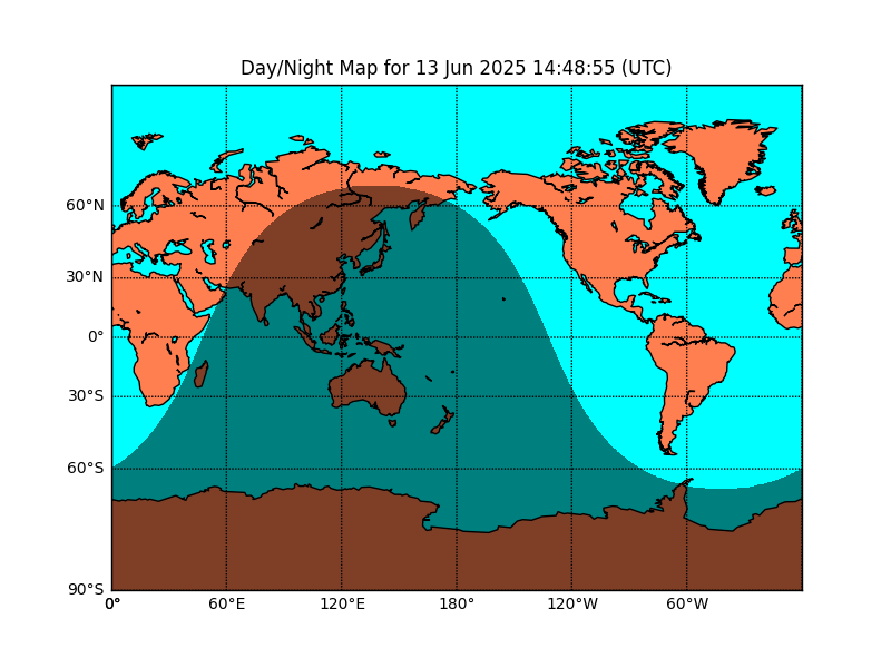
在地图上绘制昼夜晨昏线。
import numpy as np
from mpl_toolkits.basemap import Basemap
import matplotlib.pyplot as plt
from datetime import datetime
# miller projection
map = Basemap(projection='mill',lon_0=180)
# plot coastlines, draw label meridians and parallels.
map.drawcoastlines()
map.drawparallels(np.arange(-90,90,30),labels=[1,0,0,0])
map.drawmeridians(np.arange(map.lonmin,map.lonmax+30,60),labels=[0,0,0,1])
# fill continents 'coral' (with zorder=0), color wet areas 'aqua'
map.drawmapboundary(fill_color='aqua')
map.fillcontinents(color='coral',lake_color='aqua')
# shade the night areas, with alpha transparency so the
# map shows through. Use current time in UTC.
date = datetime.utcnow()
CS=map.nightshade(date)
plt.title('Day/Night Map for %s (UTC)' % date.strftime("%d %b %Y %H:%M:%S"))
plt.show()
(源代码)